In this blog post, we will apply Vintage Sparse PCA (vsp) (Rohe and Zeng, 2020) on the microbiome data collected from the Earth Microbiome Project (EMP) to explore the microbiome patterns worldwide.
-
Data description
Earth Microbiome Project (EMP) uses a systematic approach to characterize microbial taxonomic and functional diversity across different environments and humankind (Thomson et al., 2017). EMP comprises 27,751 samples from 97 studies with microbial data representing 16S rRNA amplicon sequencing, metagenomes, and metabolomics. For this blog, we used a rarefied subset data composed of 2,000 samples representing all environments and humankind microbiomes created by EMP. The dataset is divided by (1) an operational taxonomic unit (OTU) table, (2) and sample table, and (3) a metadata table. Below is the column information for each table.
(1) OTU table: ID, Sequence, Kingdom, Phylum, Class, Order, Family, Genus, and Species.
(2) The sample table contains ID and Sample Name.
(3) Metadata table: 76 environmental information from each sample. For this blog, we used Sample ID, Environment Biome, and Environment Feature. -
Data manipulation
To represent the biomes as a graph, we built an OTU-sample bipartite adjacency matrix, named A. For this, we used the R Matrix package. Aij = x was composed by OTUs as i, samples as j, and the number of OTUs observed in the sample as x. The dimensions of the A matrix was 155,002 rows and 2,000 columns. To examine the A matrix, we did a histogram and found that some OTUs were more abundant than the other, which is natural in microbial ecosystems.
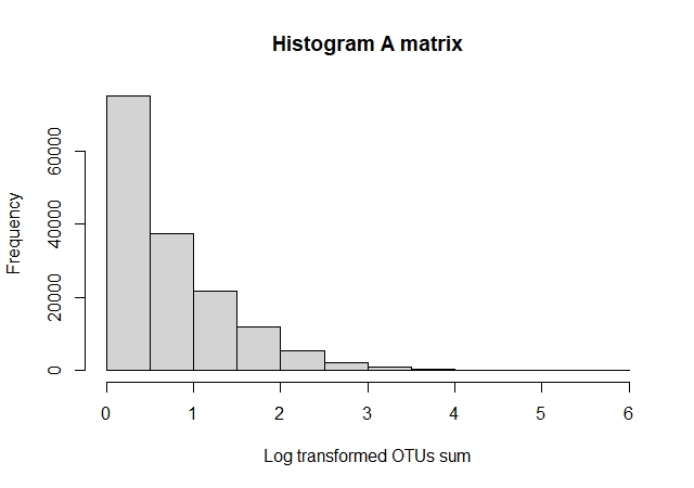
Figure 1. OTU amount distributionTo make the data more manageable, we subsetted the data for three prominent phyla: Proteobacteria, Bacteroidetes, and Firmicutes. Also, we chose the OTUs with a prevalence of at least ten samples. Then, we made a matrix with the selected phyla and did square root transformation for variance stabilization, named A.sel. The A.sel matrix had a dimension of 8,263 rows and 2,000 columns and a right-tailed distribution.
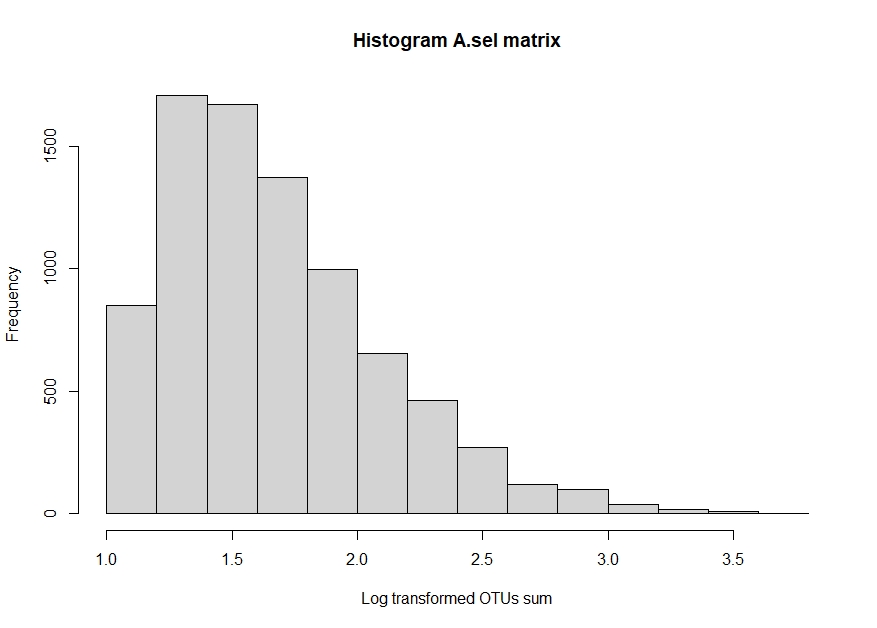
Figure 2. Subset OTU amount distribution (with variance stabilization) - Clustering Sample sites into communities
We used Vintage Sparse PCA (vsp) to cluster samples into 20 communities using the R vsp package. It is expected that sample sites with a similar beta-diversity (i.e. consists of similar numbers of specific OTUs) will be clustered together. The vsp function requires an adjacency matrix, the number of factors to be calculated, and whether to center/scale or not. As we hope to estimate the beta’s in Latent Dirichlet Allocation (LDA) model, we will do vsp with centered and scaled adjacency matrix. Further, we will examine several diagnosis plots to check the vsp result.
(1) VSP with centering, scaling, and rescalingfa_center<-vsp(A.sel,rank = 20,center = TRUE,scale = TRUE,rescale = TRUE,recenter = FALSE)(2) Diagnosis plot
- Check that streaks are well-aligned with factors (use y-pair because we are looking at sample clusters)
 #plot the first 10 factors
 plot_varimax_y_pairs(fa_center,1:10)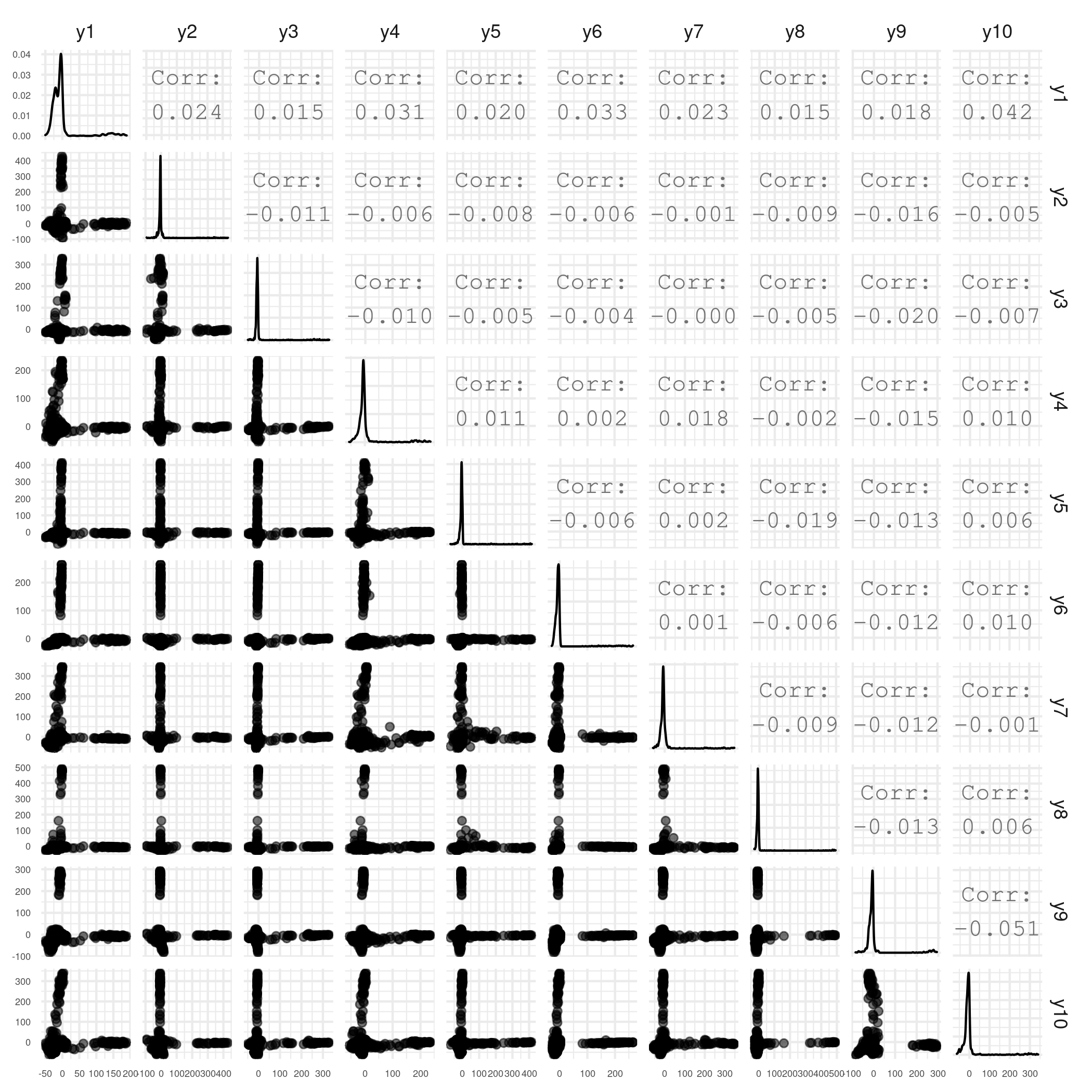
Figure 3. Sample-wise factor pair plot - Check the B matrix is roughly diagonal: if the purple encodings mainly exist on the diagonal, we say that the B matrix is a diagonal matrix.
plot_mixing_matrix(fa_center)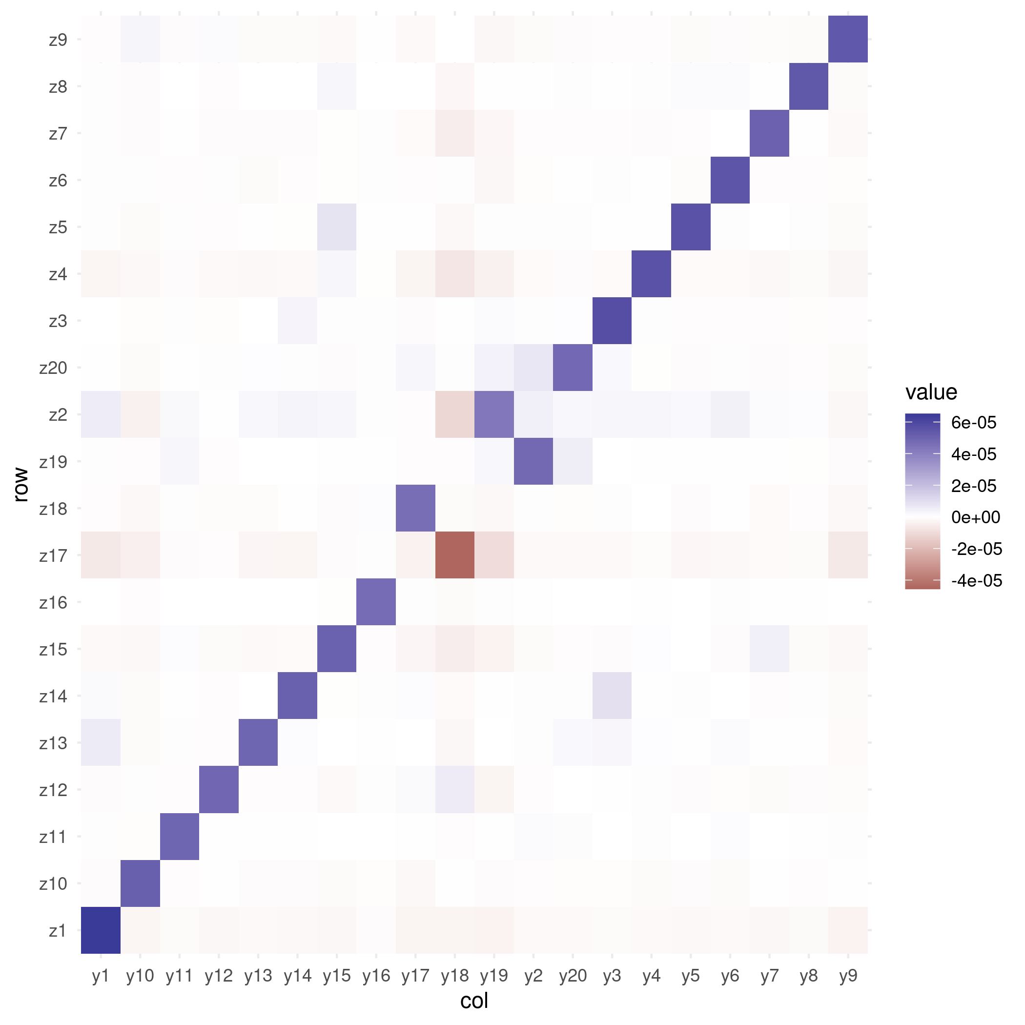
Figure 4. B matrix diagonality
(3) Reason for chosing rank=20
Based on two reasons: first, according to the original EMP paper (Thomson et al., 2017), its standard sample report regulation includes 17 levels of environmental features. Second, based on the scree plot, there is a drop around 20.
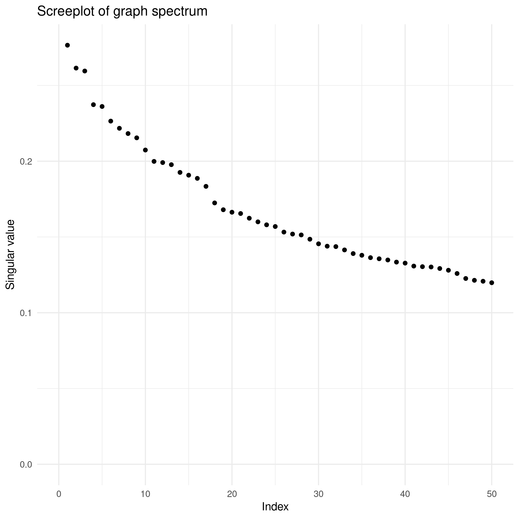
Figure 5. Screeplot
- Check that streaks are well-aligned with factors (use y-pair because we are looking at sample clusters)
- Contextualizing clusters
For contextualizing the clusters, we used external sample environmental information and the “best feature function” or bff from the vsp R-package. bff is similar as the traditinoal tf-idf method, which finds the most associated feature for each cluster. The bff function requires:
(1) loadings: an n by k matrix of the weights that indicates how important “i”th sample is for the “j”th cluster
(2) features: an n by d matrix that contans features for each node in the network (called sample_meta_mtx)
(3) num_best: a number indicating how many features for differentiating between loadings we wanted
For exploratoin purpose (and fun!), we contexualized the clusters respectively with two kinds of external feature data, one is environmental biome tpye, and the other is environmental feature type.The biome data characterized the environment as a habitat related to plants, animals, and climate (e.g., Tropical forest, temperate grassland). The feature data described the environment as a particular component of the environment where the sample was collected (e.g. soil, coral, bay).
Each parameter we used are, loadings: the Y matrix frmo vsp result; features: either environmental biome (call eenv_biome) or envieonmental feature (called env_feature) type; num_best: 10.library("Matrix") sample_meta_mtx=cast_sparse(sample_meta_ID,ID,env_feature)#create sparse matrix for features sample_meta_mtx2=cast_sparse(sample_meta_ID,ID,env_biome)#create sparse matrix for biomes #characterize clusters feature= bff(fa_center$Y, sample_meta_mtx,10) biome= bff(fa_center$Y, sample_meta_mtx2,10)As a result, we got the following characterizations.
Table 1. Contextualization: with environmental bimoe type
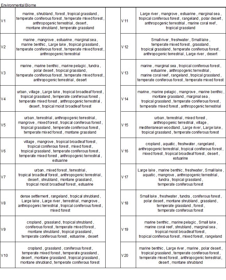
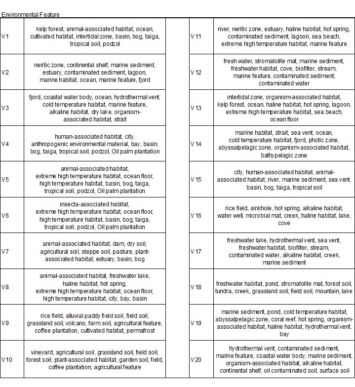
Table 2. Contextualization: with environmental feture
To interpret the bff results, we need to first understand how env_biome and env_feature related with each other; then, we can describe the sample sites representing each cluster. Contextualizing with the environmental biomes resulted in more complexity. This complexity has to do with the more general information/fewer levels provided in the env_biome variables. However, we can see some interesting groups. For example, V5 represents a cluster where many of the grouped sample sites cnotain disturbed microbiomes. Cluster V11 shows samples with high temperature boimes, high salinity biomes, or high ionic activity biomes in the water or the soil. Cluster 16 shows a similar trait as V11. The difference between V11 and V16 is that there are more biomes related to water in V16. Overall, biomes may be a too general attribute for such diverse data, but many biome types were successful in specifying something about the cluster.
The environmental features were more effective in describing the clustering. For example, V5 represents sample sites related to agriculture and farming. In some ways, it is similar to the biomes characterization, however, with more detail. Cluster V11 shows features related to water, hot climates, and contaminated sediments, which was also very similar to what we interpreted from the biomes. However, the features in V16 do not seem so similar to cluster V11, like in the biomes. Cluster V16 in the features describe a cluster of samples that associate with water or low oxygen environments. In sum, both biome and features provide characterization to the clustering. However, biomes may be too general to understand the microbiome of each cluster in our analysis. The features of the environment were more informative of the sample site clusterings. - Estimate cluster composition
To further evaluate the cluster composition, LDA model is commonly used. As vsp can estimate the beta’s in the LDA model (Rohe and Zeng, 2020), below we show the calculation steps and results.
(1) Use the Z matrix from centered, scaled, and rescaled vsp result (Z=fa_center$Z)
(2) Calculate phi=Z’A (where A is the centered adjacency matrix, called A.sel_center)A.sel_center<-A.sel entries_len<-length(A.sel_center@x) A.sel_center@x<-A.sel_center@x-(In%*%(t(In)%*%A.sel/n))[1:entries_len](3) Estimate beta
(4) Set negative betas to zero (there should only be positive values, and we regard negative ones as statistical errors)
(5) Check if each column (i.e. each community) sums up to 1phi=t(fa_center$Z)%*%A.sel_center library(wordspace) norm_phi=rowNorms(phi,method="minkowski",p=1)#calculate l1 norm for each row norm_phi_d<-diag(norm_phi) #20*20 diagonal matrix norm_phi_d_inv<-solve(norm_phi_d) #inverse of norm_phi_d beta<-t(norm_phi_d_inv%*%phi) #2000*20 beta[beta<0]=0 beta<-apply(beta,2,function(x) return(x/sum(x))) colSums(beta)#each column sums up to 1Figure 6 and Figure 7 show the cluster composition derived from the estimated beta’s. One is the biome type distribution within each flock, and the other displays in terms of environmental features. Due to space limit, for biome type distribution only those with weight > 5% are shown; for environmental features, those with weight > 6% are shown.
Overall, the estimatoins complement the results in the above table. Tables display features that are most correlated with each cluster, while estimated cluster composition allows us to see more details about how each feature occupies the cluster. For example, in Figure 6, take cluster 11 and 16 again, now their difference is clearer. Cluster 11 is mainly featured by sample sites with large river biomes; wihle cluster 16 cosnists of samples that not only have aquatic biomes but cropland and urban biomes. Over time, this cluster structure may change if purturbations are introduced. Thus, it can be a critical index for many applications, such as examining effects of wastewater treatments, medical effects in human beings, and etc.
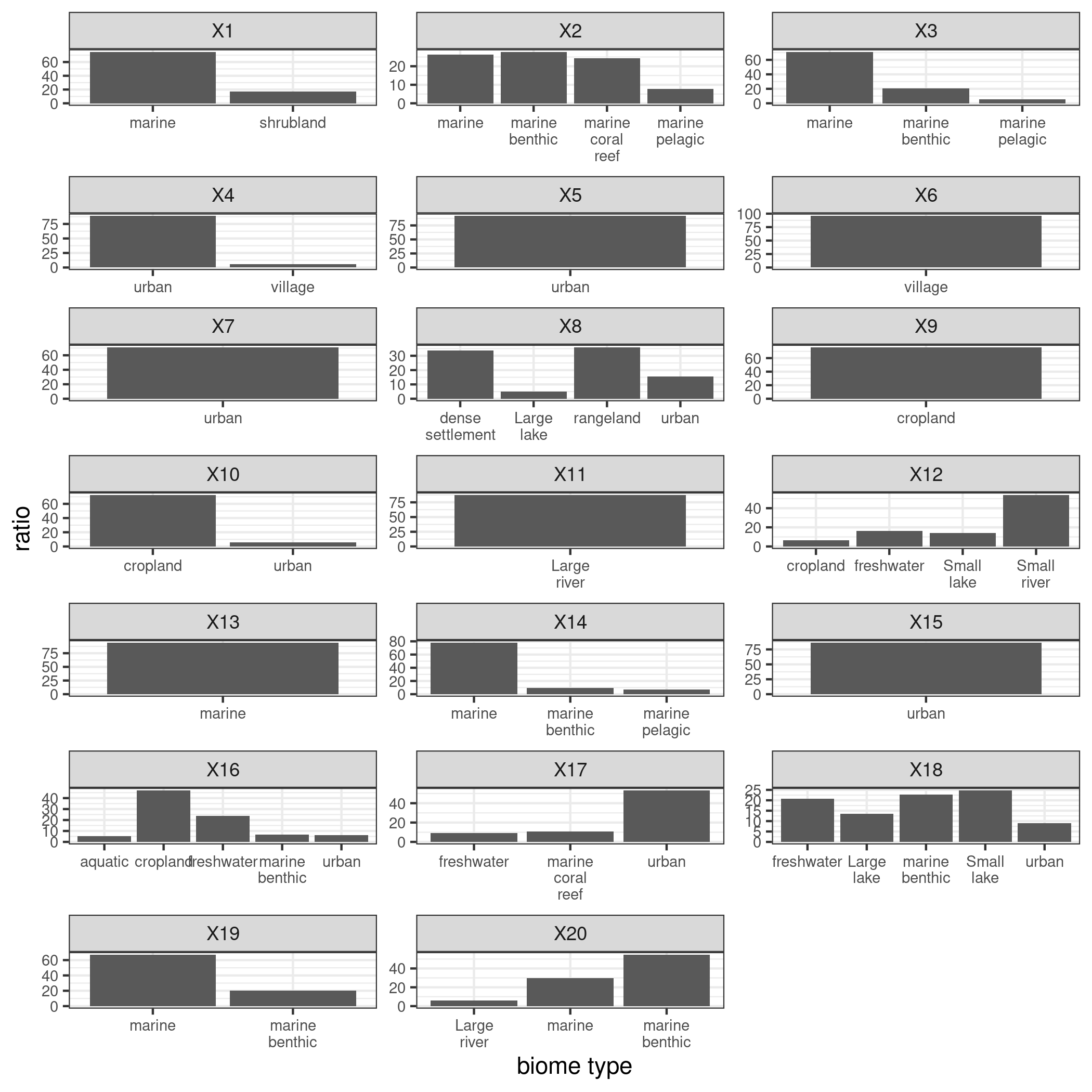
Figure 6. LDA estimation - Biome type distribution within each cluster
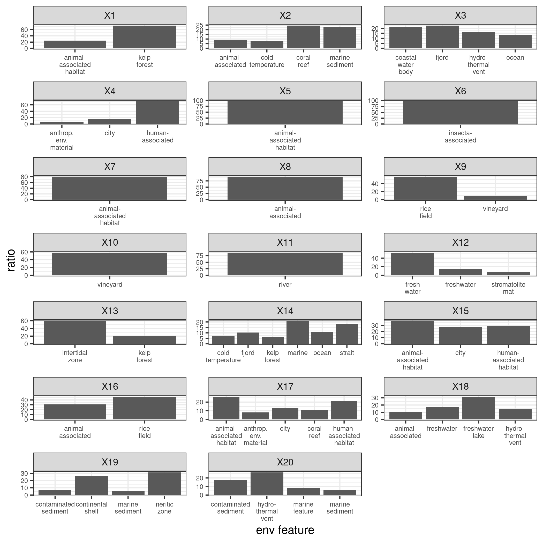
Figure 7. LDA estimation - Environmental feature type distribution within each cluster